WRDS Library [Home] Digital Library Publications Videos Card Catalog

Chapter IV
Data Analysis and Discussion of Results

DIMENSIONAL ANALYSIS
The Buckingham Pi Theorem was used to develop dimensionless parameters, the Pi (P) terms, from the variables. Five parameters are used to describe the geometry of the long crested weir: the top width of the channel (T), the width of the weir throat (L), the height of the weir crest (W), the length of the weir side crest (Sl), and the total length of the weir crest (Llcw). Variables used to describe the flow condition were the flowrate (Q), the acceleration due to gravity (g), and the head of water on the weir (H). The relationship of these variables can be described as

Q = f (g, H, T, L, W, Sl, Llcw) (2)

which indicates that the flowrate is a function of all the other parameters. The dimensionless P terms can be obtained by following the procedure outlined in Introduction to Fluid Mechanics by Fox and McDonald (1985):
1. The parameters involved are

Q g H T L W Sl Llcw n=8 parameters

(m,l,t)

Q=l³/t, g=l/t², H=l, T=l, Ll, W=l, Sl=l, Llcw=l
r=2 primary dimensions (l and t)

g=l/t² , H=l, m = r = 2 repeating parameters

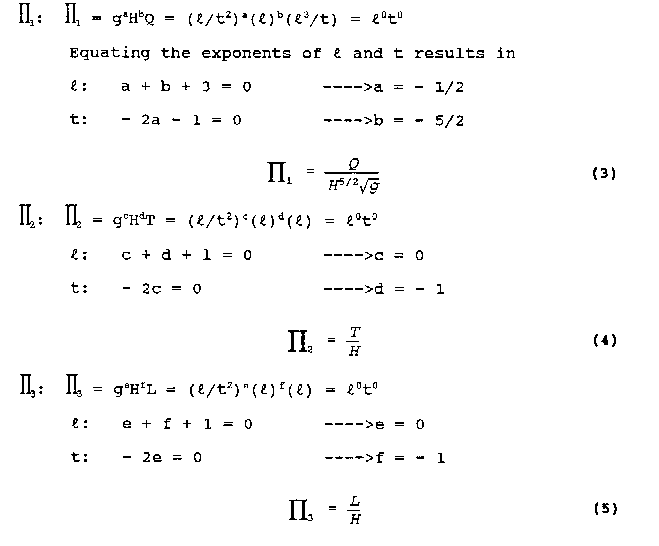
Similarly, since all the remaining parameters have units of length only, they are of the same form as P ₂ and P ₃. The remaining P terms are

P₄ = W/H (6)
P₅ = Sl/H (7)
P₆ = (Llcw)/H (8)

The functional relationship then becomes

P₁ = f (P₂, P₃, P₄, P₅, P₆) (9)

or

Q/(H^5/2 g^1/2) = f(T/H, L/H, W/H, Sl/H, Llcw/H) (10)

the actual form of this function must be determined by statistical analysis of the experimental data.

There are many possible combinations of the parameters to form dimensionless Pterms. The P ₁, term developed above using g and H as repeating parameters is Q/(H ^5/2g^l/2) and is a form of the Froude Number. If a different geometric parameter is used as a repeating parameter, then it ends up in the denominator of the dimensionless terms P ₂ through P ₆. In discussing the options of which combinations of parameters can be used as P terms, Murphy (1950, p. 37) states " ... the only restrictions placed upon the Pi terms is that they be dimensionless and independent." The quality of independence means that a P parameter considered in a problem can't be formed by the combination of the other parameters of the problem through multiplication or division. For example, the parameter L/T could not be used along with the parameters T/H and L/H because L/T = (L/H) / (T/H) . However, transformations, combinations, and substitutions are allowed on the conditions of being dimensionless and independent of the other parameters considered in the problem. Therefore, L/T could replace L/H and the parameters L/T and T/H would be independent because L/H is no longer included in the problem.

The dimensional analysis indicated that six P terms should be used to evaluate the problem, but the selection of which P terms to use involved a degree of judgment mixed with some trial and error. The equation for the flowrate of a long crested weir given by Kraatz and Mahajan (1975) is of the form

Q = C_d Llcw H^3/2 (2g)^1/2 (11)

where C_d is a discharge coefficient, Llcw is the length of the long crested weir crest, H is the head on the weir, and g is the acceleration due to gravity. This is basically the same equation as (1) but uses different letters to represent the variables. Solvin(i this equation for the coefficient of discharge, C_d, produces equation 12 which is dimensionless and similar in form to the P₁ term developed through the dimensional analysis.

C_d=Q/[Llcw H^3/2 (2g)^1/2] (12)

Because C_d is dimensionless, independent, and similar in form to P ₁, it can be substituted for P ₁ in the evaluation of the problem. This allows the evaluation of the coefficient of discharge as a function of the geometry parameters:

C_d = f (P ₂, P ₃, P ₄, P ₅, P ₆) (13)

A multivariable linear regression was done to relate C_d to the other parameters. The repeating parameter with just the dimension of length was varied to produce different terms of P₂ through P ₆. The r² fit of the different linear regressions was as follows:

C_d = f (W/H, L/H, T/H, Sl/H, Llcw/H); r² = 55.5% (14)

C_d = f (H/W, L/W, T/W, Sl/W, Llcw/W); r² = 77.3% (15)

C_d = f (H/L, W/L, T/L, Sl/L, Llcw/L); r² = 80.6% (16)

C_d = f (H/T, W/T, L/T, Sl/T, Llcw/T); r² = 77.3% (17)

C_d = f (H/Sl, W/Sl, L/Sl, T/Sl, Llcw/Sl); r² = 59.8% (18)

C_d = f (H/Llcw, W/Llcw, L/Llcw, T/Llcw, Sl/Llcw); r² = 67.4% (19)

It was apparent from the linear regressions that not all of the dimensionless P parameters do an equally good job of describing C_d. For this reason, an arbitrary selection of Pi parameters would not be satisfactory. Judgment had to be used in the selection of the parameters which best described the geometry of the weir as it related to the flow conditions. Along with the judgment, there was also some trial-and-error involved in determining the final P terms and evaluating their effects on weir performance. The dimensionless parameters that were selected to be evaluated with the coefficient of discharge are explained in the following paragraphs.

A driving force behind the flow of water over the weir is the head of water on the weir, and the dimensionless term H/W appears in the Rehbock equation for sharp crested weirs (Vennard and Street 1982). The ratio of the head to the weir height has a large influence on the shape of the streamlines in the flowfield for standard sharp crested weirs. This dimensionless parameter, H/W, was selected as P ₂ for this reason (the first dimensionless term is the coefficient of discharge, C_d).

The next dimensionless parameter selected, P ₃, was L/T. This is the ratio of the long crested weir throat width to the width of the channel in which the weir is placed. This ratio gives an indication of the lateral contraction of the flow streamlines as they enter the weir. As will be shown later, the lateral contraction of the flow had a large influence on weir performance.

The dimensionless parameter H/L was selected to be P₄. This was a ratio of the head on the weir to the throat width of the weir. Along with P ₂ and P ₃ , this parameter gives an indication of the contraction of the flow entering the weir. A value of H/L near 1.0 indicated a relatively high head with a very narrow throat, and resulted in reduced performance of the weir.

The parameter Sl/Llcw was selected as P ₅, because it defines some of the geometry of the weir crest. The total length of the crest, Llcw, is given by the equation

Llcw = 2Sl + Dw, (20)

The term Sl is the side crest length, and there are two sides to each weir. The term Dw is the downstream crest width of the weir. In the case of a weir that is V-shaped in plan view, there is no downstream crest width (Dw = 0) , and the total crest length is equal to twice the length of the side crest.

The final parameter, P₆, is Llcw/L. This is a ratio of the total crest length to the width of the throat. This term is described by Walker (1987) and Hay and Taylor (1970) as a length magnification. Since a standard sharp crested contracted weir would have a crest length equal to the width of the throat, this parameter indicates how many times longer the crest of the long crested weir is than the crest of the contracted weir with the same throat width. If the throat width is equal to the channel width, then the parameter is the same (Llcw/L) , but now L = T, and the comparison of weir crest lengths would be between the long crested weir and a standard suppressed weir. Under ideal operating conditions, the flowrate of the long crested weir would be Llcw/L times greater than the flowrate for the regular weir with the same head; for example, if the crest of the long crested weir is ten times longer than the crest of the regular weir (Llcw/L = 10), then ideally the flowrate over the long crested weir should be ten times greater than the flowrate over the regular weir with the same head. The experimental results showed that the flow magnification was often much less than the length magnification, but this parameter was still useful in describing the behavior of the weir.

EQUATION FOR C_d

Once the P terms were determined, the data could be analyzed and an equation for C_d be developed. As shown in (13), the symbolic relationship of the parameters is

C_d = f(P₂, P₃, P₄, P₅, P₆),

Q/[Llcw H^3/2 (2g)^1/2] = f (H/W, L/T, H/L, Sl/Llcw, Llcw/L) (21)

The objective was to develop an equation for C_d, and several forms of equations were tried. The first form of equation was a simple linear relationship between C_d and the rest of the parameters:

C_d = a + bP₂ + cP₃ + dP₄ +eP₅ + fP₆, (22)

where a through f are regression coefficients from a multivariable linear regression of the data. The second form of equation is a second-order polynomial equation which starts the same as the linear equation but adds the P terms raised to the second power:

C_d = a + bP₂ + c P₃ + dP₄ + e P₅ + fP₆ + gP₂² + h P₃² + i P₄² + j P₅² + k P₆², (23)

where the letters a through k represent regression constants (the constants a through f in this polynomial will be different from those given in the linear equation above) . The other form of equation is a power function:

C_d = aP₂^b P₃^c P₄^d P₅^e P₆^f, (24)

where again the letters a through f represent constants. The constants of the power function are found by taking the logs of the data and by doing a linear regression on the logs as shown in equation 25:

logC_d = loga + b logP₂ + c logP₃ + d logP₄ + e logP₅ + f logP₆, (25)

Although the number of terms involved makes the equations somewhat long, they are all simple to use.

The analysis of the data was limited to these three types of equations for several reasons. When starting the data analysis, it was not known what type of equation would best fit the data. one of the characteristics desired in the prediction equation for C_d was simplicity of both form and use. The linear and power functions are both simple in form and simple to use once the coefficients are known. The second-order polynomial equation is a little more cumbersome because of the 11 terms, but it is still simple to use. Of course, another characteristic that was desired was a high correlation coefficient (r²) which indicates how well the data fit the relationship. As the following data analysis shows, all of these three types of equations produced r² values above 80 %. The third-order polynomial was also tried during the data analysis, and it produced a better r² than any of the other three types of equations. However, the cubic type equation was very cumbersome, and the one or two percent improvement in the r² appeared to be the result of the added degrees of freedom rather than actually being a better prediction equation.

The regressions were first performed on the entire data set. All of the data regressions and analysis was performed using MINITAB statistical software. The multivariable linear regression yielded the following equation which had an r² value of 85.5 %:

C_d = 0.618 - 0.346P₂ + 0.0143P₃ - 0.188P₄ - 0.181P₅ - 0.0107P₆, (26)

The second-order polynomial equation gave an r² of 92.0 % with:

C_d = 0.296 - 0.482P₂ - 0.236P₃ - 0.808P₄ + 2.29P₅ - 0.0223P₆
+ 0.797P₂² + 0.104P₃² + 0.485P₄² - 2.l93P₅² + 0.000694P₆², (27)

The evaluation of a power function for the data gave and r² fit of 81.5 %:

logC_d = -0.554 - 0.2691logP₂ + 0.2231logP₃ - 0.2061logP₅ - 0.1471logP₆

The logP₄ term was highly correlated with the other variables, and MINITAB automatically removed it from the equation. These values correspond to the following power function:

C_d = 0.2795P₂^-0.269 P₃^0.223 P₅^-0.206 P₆^-0.147, (28)

These initial equations resulted from the analysis of the entire set of experimental data and may be considered general equations for the entire set of experiments.

Some recommendations by French (1985) for various standard sharp crested weirs indicate that limitations should be placed on the operation of the weir. One of the recommendations is that the lower limit of head on the weir be about 0.10 feet because viscous and surface tension effects start to have a large influence at heads lower than this. In the experiments with the long crested weirs in the laboratory, the measurements of minimum head and flowrate were taken at a flow just greater than the flow at which the nappe would start clinging to the weir crest. These measurements were at heads less than 0.10 feet, and some of the experimental C_d values were very high which agrees with French's comments. The upper limit of the head to crest height ratio for fully contracted weirs was recommended to be 0.5 (French 1985). Most of the laboratory measurements were made for H/W <= 0.5, but there were a few measurements that were greater than this upper limit. If the limitations of H/W <= 0.5 and the minimum H = 0.10 feet are applied to the experimental data by deleting all the data that does not fall within these bounds, the following equations result and are applicable to all the weirs tested. For linear regression the r² = 93.4%, and the equation is

C_d = 0.543 - 0.217P₂ + 0.0597P₃ - 0.163P₄ - 0.193P₅ - 0.00953P₆, (29)

After the linear regression was done, the data was fit to a second-order polynomial equation which gave an r² = 96.6%:

C_d = 0.366 - 0.193P₂ - 0.247P₃ - 0.727P₄ + 1.65P₅ - 0.0212P₆
+ 0.351P₂² + 0.129P₃² + 0.413P₄² - 2.17P₅² + 0.00065P₆², (30)

The power function had an r² = 84.8% with:

C_d = 0.2793P₂^-0.289 P₃^0.247 P₅^-0.256 P₆^-0.179, (31)

The polynomial again provides the best fit of the data, and all of these equations showed an improvement in the r² values over the general equations produced from the entire data set.

The following pages contain plots of the actual test flowrates in the weirs versus the flowrates that are predicted by applying equations (29) and (30) to the experimental data. Figures 8, 10, 12, and 14 show the plots of Qa vs. Qp where Qp, the predicted flowrate, is predicted using equation (11) with equation (29) being used to calculate the value of C_d, and Qa is the actual flowrate taken from the experimental data. Figures 9, 11, 13, and 15 show the plots of Qa vs. Qp where Qp is predicted using equation (11) with equation (30) used to calculate the value of C_d. The two graphs on each page give a comparison of the predicted flowrates using the C_d values determined by the linear and the second order polynomial equations. The figure at the top of the page used the linear equation to predict C_d, while the values in the figure at the bottom of the page use the second-order polynomial equation to calculate C_d for the same weirs.

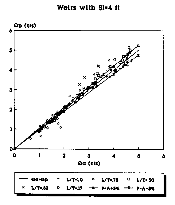
Figure 8. Actual vs Predicted Flowrate Using the Linear Equation for All Wiers (Sl=4 ft.).

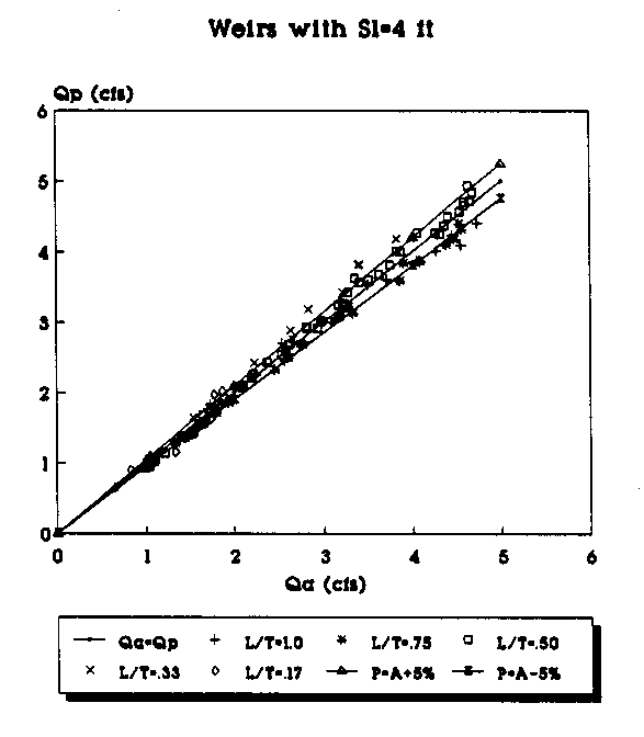
Figure 9. Actual vs Predicted Flowrate Using the 2nd Order Equation for All Weirs (Sl=4 ft.).

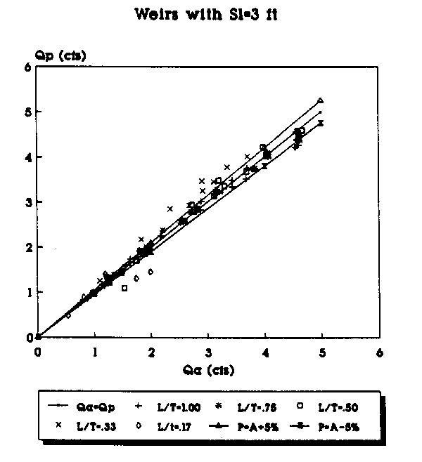
Figure 10. Actual vs Predicted Flowrate Using the Linear Equation for All Weirs (Sl=3 ft.).

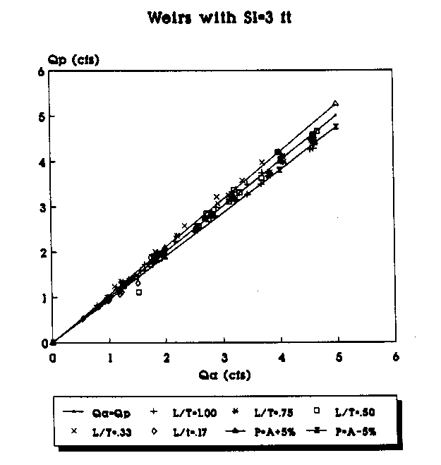
Figure 11. Actual vs Predicted Flowrate Using the 2nd Order Equation for All Weirs (Sl=3 ft.).

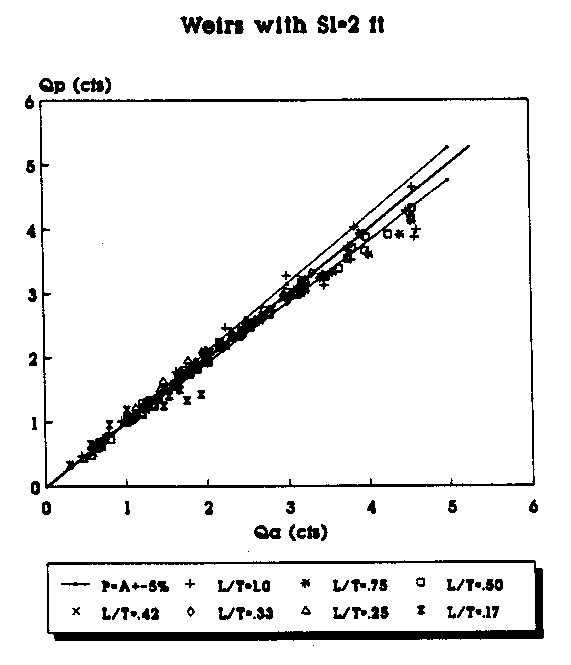
Figure 12. Actual vs Predicted Flowrate Using the Linear Equation for All Wiers (Sl=2 ft.).

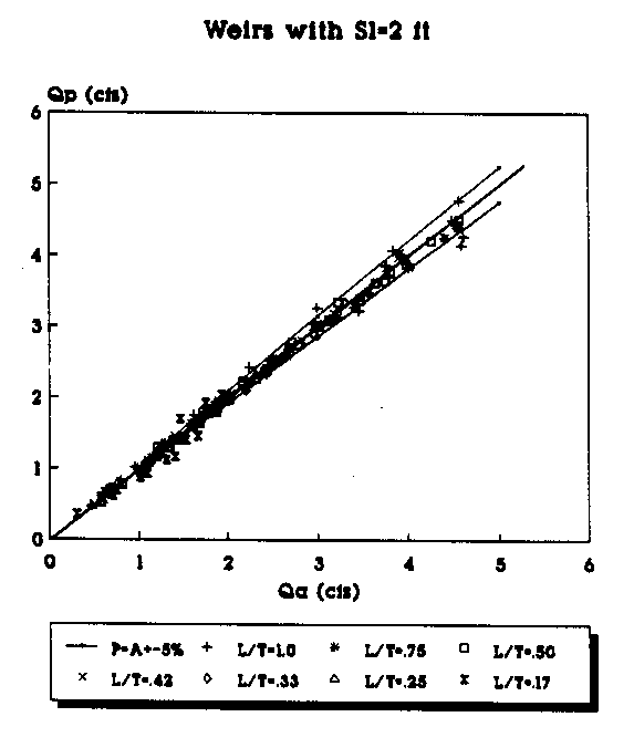
Figure 13. Actual vs Predicted Flowrate Using the 2nd Order Equation for All Weirs (Sl=2 ft.).

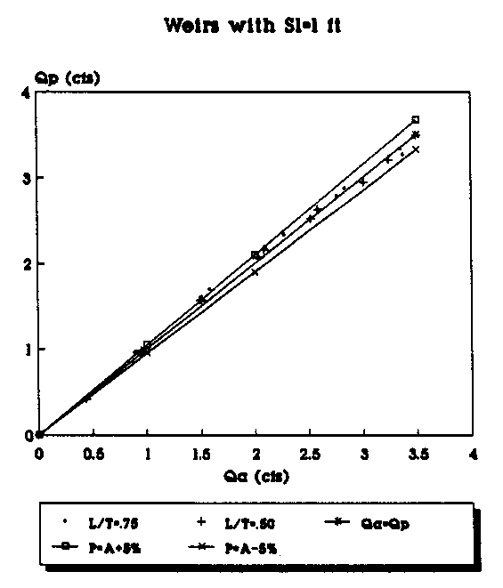
Figure 14. Actual vs Predicted Flowrate Using the Linear Equation for All Weirs (Sl=1 ft.).

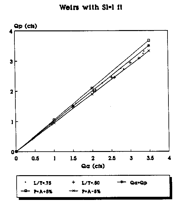
Figure 15. Actual vs Predicted Flowrate Using the 2nd Order Equation for All Weirs (Sl=1 ft.).

To plot the graphs, the data were segregated according to the length of the weir side crest, Sl. Weirs with different throat widths were plotted as a different series and are represented by a different symbol in the legend of the figures. For example, in Figure 6 the data points (Qa,Qp) for all of the suppressed weirs (L/T=1.0) with Sl=4 ft are represented by the "+" symbol. Each figure has a line which represents where the predicted flowrate would be equal to the actual measured flowrate. The objective is, of course, to get the predicted flowrate as close to the actual flowrate as possible. The figures also have a curve above and below the Qa=Qp line. The top curve (P=A+5%) shows the curve of predicted values 5 percent above the actual flowrate. The bottom curve (P=A-5%) shows the curve of the predicted values 5 percent below the actual flowrate. The area between the curves shows the range of the actual flowrate plus or minus 5 percent.

By plotting the data in groups according to Sl and the L/T values, some trends in the predicted flowrates become apparent. The predictions made with the second order polynomials consistently provided the predictions closest to the Qa=Qp line. As the L/T ratio decreases, the flowrate predictions tend to be further from the Qa=Qp line for both the linear and second-order polynomial equations; however, the fit improves with the second-order polynomial predicted flowrates even for the small L/T ratios. With the second- order polynomial equations, the bulk of the data points consistently fall on or within 5 percent of the actual values. Another trend appears to be that as the weir side length decreases, the predictions seem to be consistently closer to the actual values.

The range of the data represented by the graphs in Figures 8 - 15 can be defined by the ranges of the P terms. The term P₂ = H/W had a range of 0. 5 to 0. 1. The term P ₃ = L/T had a range of 1.0 with a fully suppressed weir to 0.17 with the 6 inch throat width. The term P₄ = H/L had a range of approximately 1. 0 (6 inches of head in a 6 inch throat) to approximately 0.033 (0.1 ft of head in the 3.0 ft throat of a suppressed weir). The P₅ = Sl/Llcw term had a high value of 0.5 for triangular plan view weirs and a low of 0.286 for the weirs with a Sl = 1 ft and Llcw =.3.5 ft. The final term, P₆ = Llcw/L, had a high of 17 for the weir with Llcw=8.5 ft and L=0.5 ft and a low of 1.44 for the weir with Llcw=3.25 ft and L=2.25 ft. The laboratory data in the appendix provide the actual weir geometries.

Although the linear and second-order polynomial equations show a good fit of the data taken from all of the weirs tested, the validity of some of the data obtained while testing the suppressed long crested weirs may be questionable. The curves for the coefficient of discharge for these weirs did not follow the general pattern of the Cd curves for the contracted weirs (Figure 16).

Figure 16. Comparison of Contracted and Suppressed C_d Curves.

This difference in the C_d curves may be due to a phenomena similar to that which caused the humps in the performance curves of the labyrinth weirs where the initial loss of ventilation in the nappe due to downstream interference gave a small increase in performance and then a consistent decrease in performance with increasing head (Hay and Taylor 1970). More flow interference with the channel sidewalls was observed with the suppressed weirs than any of the other weirs because the weir side crests were against the walls of the channel. However, limitations in the laboratory facilities did not allow the testing to see if there was an actual hump in the performance curve similar to the labyrinth weirs. Another aspect of the experiment that may or may not have caused error in the data was the aeration of the nappe for the suppressed weirs. Ventilation of the nappe was provided by a series of plastic tubes arranged in such a way as to avoid disturbing the flow over the crest. Air behind the nappe was readily apparent during the experiments, but occasionally the ventilation tubes filled with water and the air supply was limited. Although visual observation of the nappe was enough to verify if it was aerated or not, the degree of aeration was not readily apparent. If during various experiments with the suppressed weirs, the ventilation was not adequate to provide full aeration, then the pressure on the underside of the nappe would have been less than atmospheric. Such a decrease in pressure behind the nappe would have caused increased curvature of the nappe and increased discharge over the weir (French 1985).

In cases where long crested weirs that would be used for flow measurement are not suppressed weirs, it may be preferrable to use an equation developed from only the contracted weir data. The range of contractions that were tested are .167 <= L/T <= .75, where L/T is the ratio of the weir throat width to the channel width. If the suppressed weir data is deleted from the entire data set, as well as the data for H < 0.10 ft and H/W > 0.5, then the analysis of the remaining data for all of the contracted weirs provides the following equations:

C_d = 0.558 - 0.277P₂ + 0.0839P₃ - 0.123P₄ - 0.232P₅ - 0.00983P₆ (32)

This linear regression equation has an r² = 93.7%. The second-order polynomial below gives an r² = 97.4%:

C_d = 0.287 - 0.350P₂ - 0.211P₃ - 0.585P₄ + 2.06P₅ - 0.0217P₆
+ 0.475P₂² + 0.136P₃² + 0.323P₄² - 2.72P₅² + 0.000642P₆², (33)

The power function had an r² = 87.7%.

C_d = 0.2983P₂^-0.342 P₃^0.293 P₅^-0.197 P₆^-0.201, (34)

Plots of Qa vs. Qp for the data using equations (32) and (33) appear on the following pages. Figures 17 - 24 use the contracted weir data, meaning that all of the weirs have a contraction at the throat so that L/T < 1.0. Similar to the graphs shown previously, the Qa=Qp line represents the set of values where the predicted and actual flowrates would be equal. The range of plus or minus 5 percent is also shown on these graphs

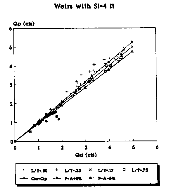
Figure 17. Actual vs Predicted Flowrate Using the Linear Equation for Contracted Weirs (Sl=4 ft.).

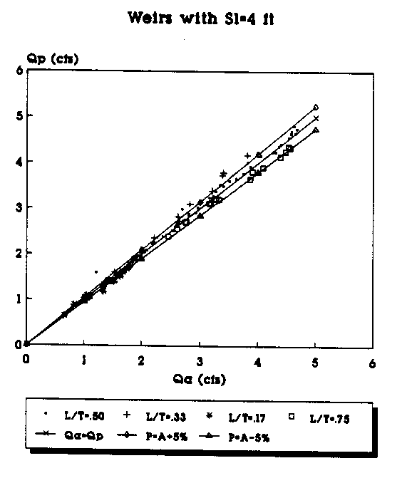
Figure 18. Actual vs Predicted Flowrate Using the 2nd Order Equation for Contracted Weirs (Sl=4 ft.).

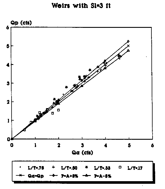
Figure 19. Actual vs Predicted Flowrate Using the Linear Equation for Contracted Weirs (Sl=3 ft.).

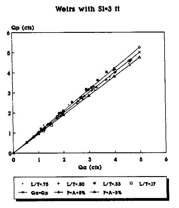
Figure 20. Actual vs Predicted Flowrate Using the 2nd Order Equation for Contracted Weirs (Sl=3 ft.).

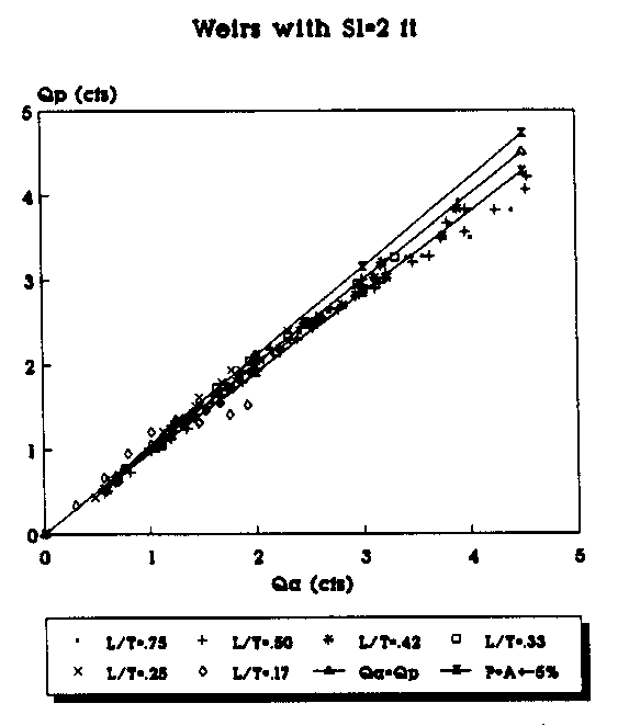
Figure 21. Actual vs Predicted Flowrate Using the Linear Equation for Contracted Weirs (Sl=2 ft.).

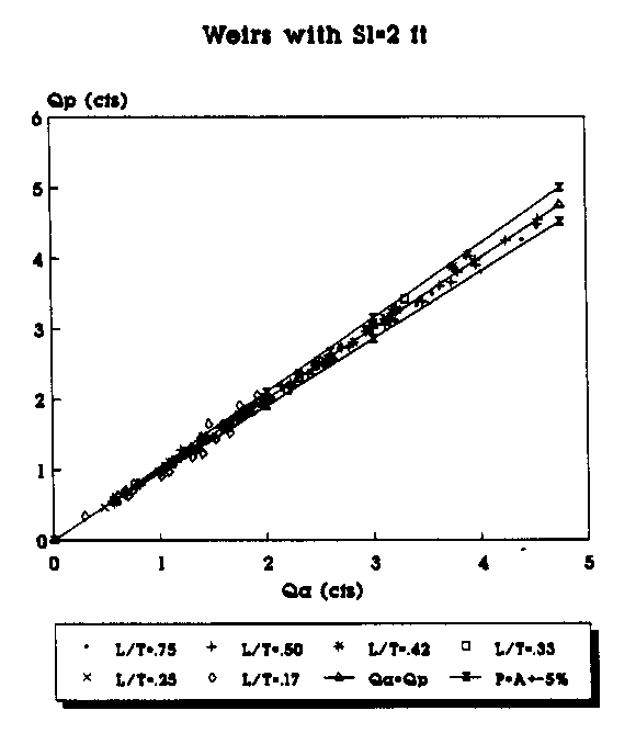
Figure 22. Actual vs Predicted Flowrate Using the 2nd Order Equation for Contracted Weirs (Sl=2 ft.).

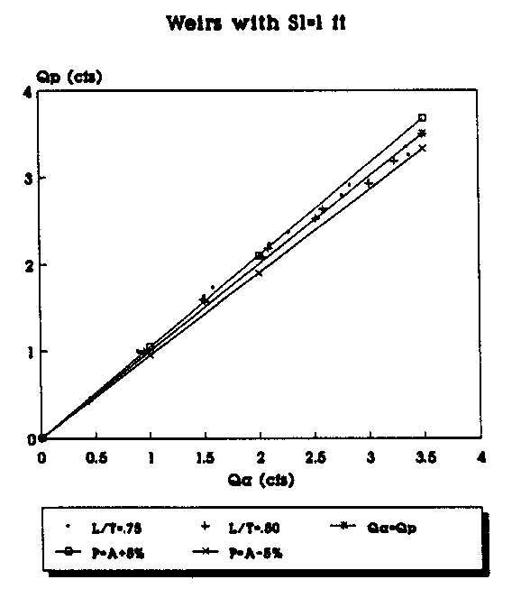
Figure 23. Actual vs Predicted Flowrate Using the Linear Equation for Contracted Weirs (Sl=1 ft.).

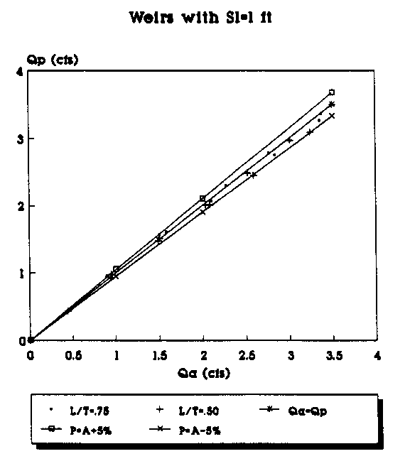
Figure 24. Actual vs Predicted Flowrate Using the 2nd Order Equation for Contracted Weirs (Sl=1 ft.).

It appears that for all of the data groups considered, the polynomial equations provided the best fit based on the r² values and the Qa vs. Qp graphs; the linear equations had the next best fit, and the power function had the lowest r² values of the three types of equations. The r² values also increased as the application of the equations became more specific and limitations were placed on which data were used in the analysis. The predictions generally tended to be better for the higher L/T values and the lower Llcw/L values. The weirs with the higher values of L/T were more effective at discharging larger flowrates with lower heads; for example, the weirs with L/T = 0.75 discharged almost double the flow of the weirs with L/T = 0.17 with nearly the same head and crest length. This is apparently due to the degree of contraction of the flow streamlines and how much of the flow has to make 90° changes in direction to discharge over the weir crest.

APPLICATION OF THE EQUATIONS
Because the coefficient of discharge is expressed in terms of head and the geometric parameters, the equations allow the flexibility of being applicable to many different configurations of weirs, so long as they are of the general shape of the so-called duckbill wiers. No diagonal or labyrinth weirs were tested, so the equations do not apply to these types of long crested weirs. Also, weirs with a crest that is rounded or something other than sharp would have different discharge characteristics than the sharp crested weirs tested, so the equations from this thesis would not apply. Although the first set of equations were developed from the entire set of data from the 67 weirs tested, it is recommended that the the second set of equations for all the weirs be used for general design purposes for suppressed weirs. The reason for selecting the second set of equations rather than the first is because of the limitations placed on the data of having H not less than 0.10 feet and of not operating the weir under H/W ratios greater than 0.5. These restrictions make the range of the data more specific, give a better r² fit, and would likely be more consistent with the actual operating limits of a weir used in the field. If only contracted weirs are being designed, it is recommended that only the last set of equations be used because they were developed specifically from just the contracted weir data.

A procedure similar to that presented by Walker (1987) could be used to design long crested weirs. The first step is to determine the maximum allowable water surface elevation either by an analysis of the effects of a backwater curve on upstream structures in the channel or by taking the total depth of the canal and subtracting the required allowance for freeboard. The minimum weir height may then be determined by the minimum head required on the turnout and by the depth of flow downstream of the weir. The weir must be tall enough to maintain the required head on the turnout even at minimum flow in the canal and also be tall enough to operate under free flow conditions with the nappe fully aerated when the downstream water surface is highest during peak canal flows.

The third step is determining the maximum weir head, which is done by subtracting the weir height from the maximum allowable water surface elevation. According to the limitations given by French (1985), the recommended minimum weir head on a weir used for flow measurement should not be less than 0.10 foot. The design head should be somewhere between these maximum and minimum weir heads. The designer should know the maximum and minimum flows that are likely to occur in the canal, and the designer should also determine how much fluctuation in the turnout is acceptable, as this value will influence the limiting range of design heads on the long crested weir.

The designer should then decide on the throat width of the weir (which will give the term L/T) ; the larger values of L/T tended to give better performance. For the first trial, a triangular shaped weir in plan view is recommended because then the parameter Sl/Llcw is known to be 0. 5. The length of the long crested weir can be determined by using the equation

Q = C_dLlcw H^3/2 (2g)^1/2

The object of the design is usually to minimize variations in flow through the turnout while at the same time minimizing weir construction costs. A weir with a long crest will tend to provide more consistent head for the turnout, but it also costs more to build. The shorter crest may cost less, but it will not provide the same degreee of control of the flow through the turnout. The designer must use an iterative process to develop a weir design that balances performance and costs to match the specific needs of the canal system. The C_d equation that best suits the designed weir could then be used to develop rating curves for measuring flow over the structure. Once the structure is designed, the parameters Llcw, (2g) , L/T, Sl/Llcw, and Llcw/L are all constants; and by varying H in the H/W and H/L terms the predicted flowrate, Q, can be calculated for various head values.

RECOMMENDATIONS
There are a number of conditions that would be present in a field installation which were not specifically addressed in the laboratory weir tests. As noted by several authors (Kraatz and Mahajan 1975; Ackers 1978; Walker 1987), the sharp crested weirs are effective sediment traps. Especially for high weirs where the approach velocity is very small, there is great tendency for heavy sand and silt particles to settle in the channel upstream of the weir. For this reason, it is recommended that in areas where the water carries a lot of sediment either a sluice gate of some type be installed with the weir to allow the flushing of sediments from the upstream side of the weir, otherwise the canal company must install a regular schedule for clearing the accumulated sediments from behind the weir. Large deposits of sediments will certainly affect the flowfield upstream of the weir and alter the discharge characteristics. However, this research did not involve the study of the effects of a sluice gate or sediment deposits on weir performance, so their actual effects on weir discharge are unknown.

The major purpose of the long crested weirs used in irrigation canals is to maintain a fairly constant water surface elevation at turnouts. The tests of the 67 weirs in the laboratory channel involved only the weirs in the channel. There were no turnouts upstream of the weir to remove water from the channel. If the turnouts in the sides of the irrigation canal were closed, then presumably the flow conditions affecting the long crested weir in the field canal would be similar to those affecting the weirs in the laboratory channel. However, if flow is being removed from the canal through the turnouts directly upstream from the long crested weir, this removal of flow may significantly alter the flowfield and head behind the weir in such a way as to change the weir discharge characteristics. The extent of influence of the flow through the turnouts on the weir performance is unknown. This situation was not tested in these long crested weir laboratory studies, and it is recommended that any application of the C_d equations be made with this limitation in mind. Accordingly, the locations of the turnouts must be far enough upstream from the weir so that the influence of the turnouts on the flowfield in the main channel must be negligible by the time it reaches the weir.

As with any other type of flow measurement structure, whenever possible it is preferable to be able to check the calibration of the long crested weir after it has been constructed. This would allow for verification of the accuracy with which the Cd equations can predict the flowrate on a full-scale long crested weir. Once the structure has been installed and used in canal operation, a program of regular inspection and maintenance is recommended to insure proper and consistent operating conditions for the weir.

93-13 Table of Contents
Water Resources Publications List
Water Resources Data System Library | Water Resources Data System Homepage